Monte Carlo Integration

Monte Carlo integration approximates an integral by averaging random evaluations of the integrand. I derive the estimator from scratch, show why its error shrinks like $1/\sqrt{N}$, and verify everything with a worked example.

Suppose we want to compute a definite integral,

If $f$ has a closed-form antiderivative, we are done. But many interesting functions do not. A classic example is

whose antiderivative cannot be written in terms of elementary functions. The standard workaround is deterministic numerical integration, such as the trapezoidal rule, where we evaluate $f$ on a fixed grid. This works well in one dimension but degrades quickly as the dimension of the problem grows.

Monte Carlo integration takes a different approach. Rather than evaluating $f$ on a grid, we evaluate it at random points and average. At first glance this sounds like it should be worse. Why would randomness help? The answer rests on a single observation, which we can derive in a few lines.

Integrals are expectations

The key trick is to rewrite the integral in Equation 1 as an expectation. Multiply and divide the integrand by $b - a$:

This looks like a pointless manipulation until we notice that $\frac{1}{b-a}$ is exactly the probability density function of a uniform random variable $U$ on $[a, b]$. So Equation 3 is really

In words, the integral of $f$ is just the average value of $f$ under uniform sampling, scaled by the length of the interval. This reframing is the entire idea. Once an integral is an expectation, we can estimate it the way we estimate any expectation, with a sample mean.

So draw $N$ independent and identically distributed samples $U_1, \dots, U_N$ from $\text{Uniform}(a, b)$ and define the Monte Carlo estimator as

Why it works

The first thing to check is that the estimator is unbiased, meaning it is correct on average. By linearity of expectation,

Furthermore, the law of large numbers tells us that a sample mean converges to its expectation, so $\hat{I}_N \to I$ as $N \to \infty$. Unbiasedness says we are right on average, and the law of large numbers says we get closer with more samples. But how fast?

Since the $U_i$ are independent, the variance of the estimator is

where $\sigma_f^2 = \mathbb{V}[f(U)]$ is the variance of the integrand under uniform sampling. Taking a square root, the standard error is

The error therefore shrinks like $1/\sqrt{N}$​. Before moving on, Equation 8 deserves two comments.

First, notice what is not in the formula. The rate does not depend on the dimension of the problem. If we integrate over a region in $\mathbb{R}^{100}$ rather than an interval, the error still shrinks like $1/\sqrt{N}$. Deterministic grid methods cannot say the same, since covering a high-dimensional space with a grid requires exponentially many points. This is why Monte Carlo dominates in high dimensions.

Second, Equation 8 appears to have a problem. The standard error depends on $\sigma_f$, which we do not know. If we could compute expectations of $f$ under $U$ exactly, we would not need Monte Carlo in the first place. But notice that the same draws that estimate the integral also estimate $\sigma_f$, through the sample standard deviation of the $f(U_i)$ values. And since the central limit theorem tells us $\hat{I}_N$ is approximately normal for large $N$, we immediately have a confidence interval,

So a Monte Carlo estimate comes bundled with a measure of its own accuracy, at no extra cost. A deterministic grid method gives no such thing.

An example

Let’s verify all of this on Equation 2, integrating $e^{-x^2}$ over $[0, 1]$. The true value can be written using the error function,

which gives us a ground truth to compare against. The estimator in Equation 5, along with the standard error in Equation 8, takes only a few lines of code:

import numpy as np

rng = np.random.default_rng(0)

def mc_integrate(f, a, b, n, rng):
    u = rng.uniform(a, b, size=n)
    fx = f(u)
    est = (b - a) * fx.mean()
    se = (b - a) * fx.std(ddof=1) / np.sqrt(n)
    return est, se

Running it on our integrand,

from scipy import special

f = lambda x: np.exp(-x**2)
truth = np.sqrt(np.pi) / 2 * special.erf(1.0)

est, se = mc_integrate(f, 0, 1, n=10_000, rng=rng)
print(f"estimate: {est:.6f} +/- {1.96 * se:.6f}")
print(f"truth:    {truth:.6f}")

estimate: 0.747045 +/- 0.003939
truth:    0.746824

The estimate is within its own confidence interval of the truth, exactly as Equation 9 promised. But a single number hides the best part, so let’s watch the estimator work. We can compute the estimate and its confidence band after every new sample, which only requires cumulative sums:

n_max = 5000
u = rng.uniform(0, 1, size=n_max)
fx = f(u)
N = np.arange(1, n_max + 1)
 
est_N = np.cumsum(fx) / N  # (b - a) = 1 here
var_N = (np.cumsum(fx**2) / N - est_N**2) * N / np.maximum(N - 1, 1)
se_N = np.sqrt(var_N / N)

Plotting the running estimate with its 95% band gives Figure 1.

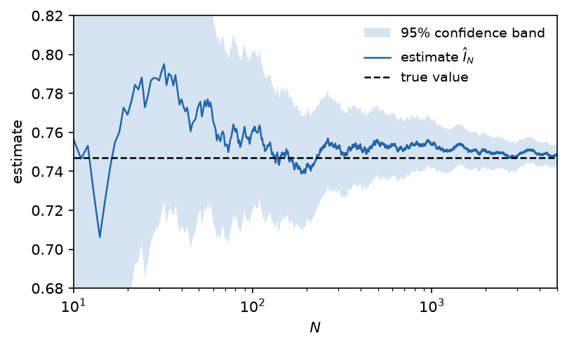
Figure 1. A single Monte Carlo run, watched as it accumulates samples. The blue line is the estimate $\hat{I}_N$ after $N$ draws, the shaded region is the confidence band from Equation 9, and the dashed line is the true value. The x-axis is logarithmic so that both the early wobble and the late settling are visible.

The figure confirms everything we derived. The estimate converges to $I$ (law of large numbers), the dashed line stays inside the band (Equation 9), and the band shrinks at the slow $1/\sqrt{N}$ rate, where each extra digit of accuracy costs $100$ times more samples.

Conclusion

Monte Carlo integration rests on a single reframing, which is that an integral is an expectation in disguise, and expectations can be estimated by sample means. Everything else follows from standard results. Unbiasedness follows from linearity, consistency from the law of large numbers, and the $1/\sqrt{N}$ error rate from the variance of a sample mean.

The lesson I take from this is not about integration. It is that a good reframing does the work of a good idea. One line of algebra in Equation 3 turned a calculus problem into an estimation problem, and estimation problems come with a complete toolkit attached.

References

Metropolis, N., & Ulam, S. (1949). The Monte Carlo method. Journal of the American Statistical Association, 44(247), 335-341.

Robert, C. P., & Casella, G. (2004). Monte Carlo Statistical Methods. Springer.